CLIP, GANs, and Art

A tutorial on how to use CLIP to guide a GAN through its latent space and produce images from text.

Each of the four images above were generated to match the text below it. By the end of this article, you will understand how these images are made, and you will have the tools to make more of these images for yourself.

This article has has 3 main sections. First, we will go over the CLIP model, which can calculate the similarity between an image and a string of text. Second, we will explore GANs, a networks architecture that allows you to generate fake images. Finally, we will look at how to combine these two models to generate art from text, as shown above.

CLIP

In the beginning of 2021, OpenAI introduced CLIP (Contrastive Language–Image Pre-training), a multimodal model that can connect text and images. Given an image-text pair, CLIP can calculate a similarity score between them.

CLIP

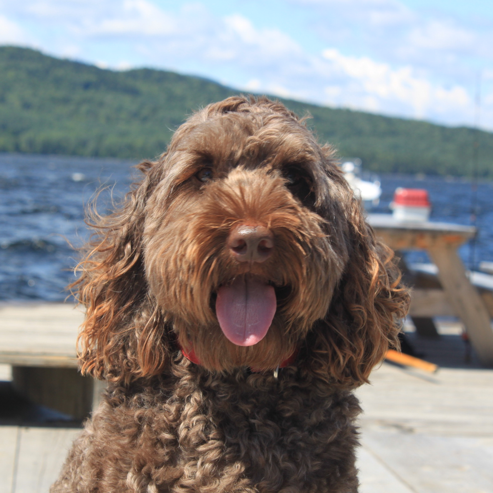
Enter some text to see how similar CLIP thinks it is to each of the 4 images.

cosine similarity: 0.34
softmax: 92.55%

[0.4,-0.2,-0.1,0.3,0.5,-0.8,0.3,0.2,0.1,0.1,0.1,-0.2,-0.1,-0.3,0.3,0.1,0.2,-0.2,0.4,-0.5,-0.4,-0.2,0.5,0.1,0,0.3,0.5,-0.4,0.1,0,-0.1,0.4,-0.3,-0.5,0.6,0.6,0,-0.1,-0.1,1.5,-0.7,-0.3,0.1,-0.1,0.1,-1.5,0.1,0.2,0.1,0.2,0.1,-0.3,0.2,0.2,0,0,0.2,0.3,-0.4,0.1,0.2,0.1,0.5,0.5,-0.2,-0.4,0.2,0.9,-0.4,-0.1,0.1,0.3,0.2,-0.2,-0.2,0,-0.2,-0.5,-0.4,-0.1,0.2,0.1,-0.4,-1,0,-0.4,0.8,-0.6,0,-0.5,-0.1,-0.6,-5.3,0.3,0,0.3,0,-0.1,-0.1,-0.4,0.2,-0.3,0.3,-0.1,0.5,0.1,1.1,0.3,-0.4,0.1,0.2,-0.7,-0.2,-0.2,0,-0.3,-0.3,-0.2,-0.1,0.1,0.5,0.6,-0.3,-0.3,0.1,-0.3,-0.2,0.4,-0.1,0.2,0.3,0,-0.4,0.8,-0.7,0.3,0.1,-0.2,0.2,0.3,-0.2,0,0.6,-0.1,-0.4,0.6,-0.1,0.4,-0.2,0.2,-0.3,0.3,-0.3,-0.3,-0.2,0,0,-0.4,-0.4,0.2,-0.3,0.2,0,0.5,0.3,-0.1,0.6,0.1,-0.2,0,0.2,-0.1,0.3,-0.2,0,-0.6,0,0,0.2,0.2,0,0.2,0.2,-0.5,0.1,-0.3,0.2,-0.5,0.1,0.1,0.1,0.3,0.2,0.2,-0.4,-0.1,0.5,-0.3,-0.4,-0.5,0.4,0.1,0,0.2,-0.5,-0.9,-0.2,0.1,-0.1,0.4,0.3,-0.2,-0.2,0,0,-0.3,-0.1,-0.1,0.8,-0.3,1.2,0.6,-0.2,0.2,0.2,0,0.1,0.1,0.2,-0.4,0.1,0.4,0.1,0.6,-0.1,-0.8,-0.4,-0.6,-0.2,0.1,0,0.2,0.3,-0.3,0,0.3,0.4,-0.2,0.5,0.3,-0.1,0.1,0.1,0.4,0.4,0.4,0.1,0,0,0.1,-0.1,0.4,0.3,-1.3,-0.1,-0.2,-0.3,0.1,-0.3,0.2,-0.1,-0.2,0.6,0.2,0.1,0,0.1,-0.3,0.1,0.3,-0.3,-0.1,-0.5,-0.4,0,0.2,-0.4,-0.2,0.2,0,0.1,0,0.2,-0.1,0.1,0.1,0.4,0.1,0.4,-0.1,0,0,-0.1,0,0.5,0.1,-0.3,0.5,0.2,-0.4,-0.7,0.8,0.8,-0.1,0.1,-0.2,0.2,-0.1,-0.4,-0.1,0.5,0,-0.3,0.8,-0.2,0.4,-0.3,0.2,-0.3,-0.2,-0.2,-0.4,0.2,-0.5,0,0.1,0.2,0.2,0.2,0,0.2,-0.4,-0.1,0.1,0.5,0,0.4,0.2,-0.6,-0.3,-0.5,-0.1,-0.2,-0.2,0.2,1.1,0.3,-0.7,0.5,0,0.9,0.2,0,0.6,-0.5,0.3,-0.2,-1,-0.3,-0.1,-0.5,-0.1,0,-0.2,0.1,0.2,1.1,0.4,0,0.3,-0.2,-0.6,0,0.2,0.2,-0.1,-0.3,0,0.5,-1.5,-0.1,-0.7,0.3,-0.3,-0.1,-0.4,-0.1,0.5,-0.5,-0.6,0.2,0.2,-0.2,-0.2,0.1,-0.3,-0.2,-0.5,0.4,-0.5,1,-0.4,-0.7,0,0,0.2,0,0.2,-0.1,0,0.3,-0.1,0.3,-1,0.3,0,-0.3,-0.1,-0.5,0,0,0.3,0,-0.6,-0.2,-0.2,-0.7,0.3,0.5,0.1,0,-0.1,-0.4,0,0.2,-0.5,-0.3,-0.1,-0.4,0.1,-0.5,-0.4,0,0,-0.2,-0.1,-0.3,-0.1,0.3,0.2,-0.5,0.1,0,0.1,0.7,0.5,0,0.3,-0.1,0.2,0.3,-0.1,-0.6,-0.5,-0.2,0.1,-0.3,0.1,-0.2,-0.2,0.3,-0.2,0,-0.2,-0.6,-0.5,-0.2,0.3,0,-0.3,-0.3,0.1,0.5,-0.3,0,-0.7,0.6,0.4,-0.4,0.1,-0.1,-0.1,-0.3,0.4,0.8,0.3,0,-0.3,-0.7,0.2,0.4,0]

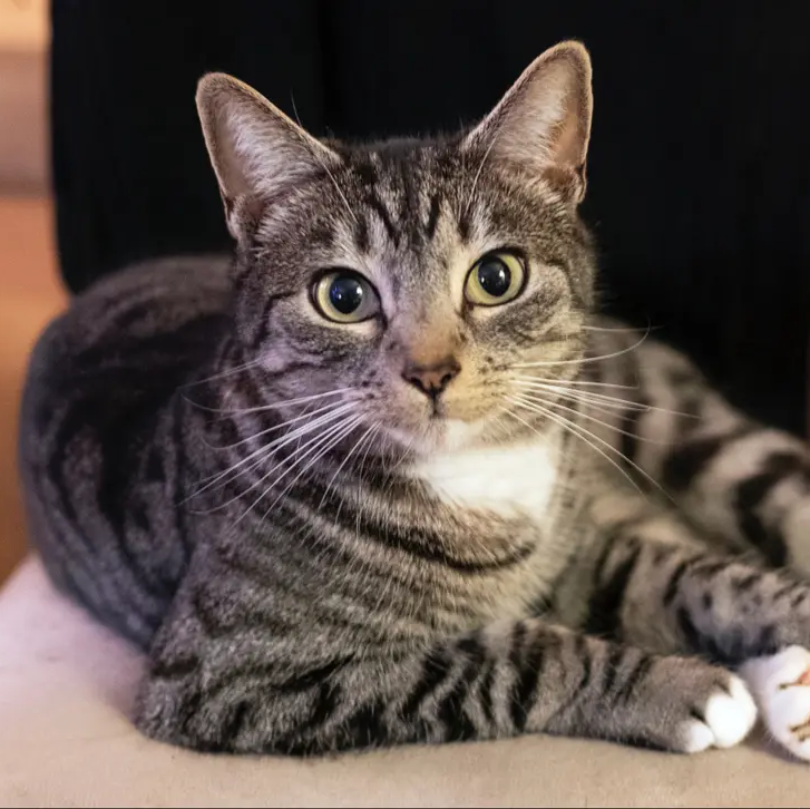
cosine similarity: 0.08
softmax: 2.31%

[-0.3,-0.2,0.1,-0.3,-0.2,-0.3,-0.2,0.7,0.8,-0.1,0.2,-0.4,0.4,-0.3,0.3,0.1,0.3,-0.1,0,0.2,-0.3,0,0.6,-0.1,-0.9,-0.2,0.5,-0.1,0,0.1,0,0.2,0,0.1,0.1,0.2,0.2,0,0.1,1.3,-0.7,-0.6,0,0.1,0,-1.1,0,0.2,0.2,-0.3,0.1,0.5,0.5,0,0.2,-0.2,0.4,0.6,-0.1,-0.2,1,-0.3,0,-0.3,-0.1,-0.6,0.1,0.6,-0.1,0.1,0,-0.3,0.1,-0.2,-0.1,-0.4,-0.1,-0.4,0.1,-0.3,-0.2,-0.4,-0.4,-0.1,0,0.2,1.4,-0.7,0.1,-0.1,0.1,-0.6,-7.1,0.3,-0.3,0.4,0,-0.5,-0.8,1.4,0.1,-0.4,-0.1,0.2,0,0.1,0.1,0.6,0.2,-0.3,-0.6,-0.4,0.5,0.3,0,0,-0.1,0.2,0.5,-0.2,0.3,0,0.2,-0.1,0.3,-0.4,0.1,0.4,-0.1,0,-0.3,-0.3,-0.1,0.8,-0.5,0.1,-0.2,-0.6,-0.2,0,0.6,0,0.4,0.5,-0.5,0.3,0.3,0.4,0.2,0.2,-0.1,0.2,-0.6,-0.1,-0.1,-0.2,0,-0.7,-0.2,-0.3,0.1,-0.1,0,-0.1,-0.1,0,0.4,0.4,0,0.1,-0.2,0.5,0.4,0.4,-0.4,0.2,0.2,0,0.6,0.4,0.1,-0.3,-0.1,0,0.2,0.2,-0.2,-0.6,0.3,-0.1,0.5,-0.4,0,-0.1,0.4,0,-0.1,-0.6,-1.7,-0.3,0,0.1,0,0.1,0.1,-0.1,-0.1,-0.1,0,0.4,-0.2,0.4,0,0.4,-0.4,-0.3,0,-0.2,1.1,-0.3,0.7,0.5,-0.3,-0.1,-0.2,0.3,0,-0.1,0,0,0.1,0,-0.4,0.3,0.3,0,0,0.1,0,-0.5,0.6,0.2,0.2,0,0.1,0.5,0.2,-1,-0.4,0.2,-0.2,0.4,0.1,-0.1,0.3,0.1,-0.2,0.1,0.1,-0.2,-0.3,0.3,0,-1.8,-0.1,-0.4,-0.1,0,-0.1,-0.1,-0.1,0,0.6,-0.2,-0.5,0,0,0.2,-0.5,0,0.2,0.3,-0.4,0,0,0.1,-0.8,-0.1,0.1,0,-0.1,-0.1,0.1,0.3,0.4,-0.1,0.3,-0.1,0.2,0.4,0.3,-0.1,0,0,0.1,-0.2,0.1,0.2,0.6,0.1,-0.6,0.3,0.8,0,0.1,0.4,0.3,-0.1,0.1,-0.1,0.5,1,-0.5,0.4,-0.1,0,-0.1,0.1,0.2,-0.1,-0.1,-0.6,0.2,-0.1,0.1,0.3,0.3,-0.1,0,0,0,-0.6,0,0.6,0.1,-0.4,0,0.3,0,-0.3,-0.7,-0.6,0.4,-0.4,-0.2,0.2,0,-0.8,0.3,0.5,-0.2,0.1,0.6,0.5,-0.1,0.2,0.1,-0.5,0.1,0,0.3,0.4,-0.1,-0.3,-0.3,-0.1,1.2,0.5,-0.3,0.3,0.3,-1.1,-0.4,-0.1,0.5,-0.2,0.2,-0.4,0.1,-0.7,0.4,-0.3,0.2,-0.2,-0.4,0,0,-0.4,-0.3,-0.2,-0.1,0.1,0,0.1,-0.3,0.1,-0.2,-0.3,0.6,-0.2,0.5,0.3,-0.3,0.1,0,-0.3,0.1,0.3,-0.2,-0.6,-0.2,0.8,0.3,-0.7,0.3,0.3,-0.3,0.1,-1.1,0.6,0.1,0.1,-0.2,0.3,-0.2,-0.4,-0.4,0.6,-0.1,-0.1,-0.2,0.4,0,0.2,0.8,-0.4,-0.2,-0.3,0.2,-0.4,0.2,-0.2,-0.2,0.7,-0.5,-0.1,0.5,0.2,0.1,0.3,-0.4,-0.3,0.2,-0.1,0.6,0.1,-0.1,-0.3,0.1,-0.3,0.7,-0.3,-0.6,-0.5,-0.6,0,-0.1,-0.1,-0.1,-0.7,0,-0.6,0,0.1,-0.6,0.3,-0.2,0,-0.5,0.1,0.4,-0.1,0.3,-0.2,0.3,0.2,0.2,0.3,0,0.1,-0.3,0.4,-0.1,0.2,0.4,-0.4,-0.3,0,-0.3,0.4,0,0.1]

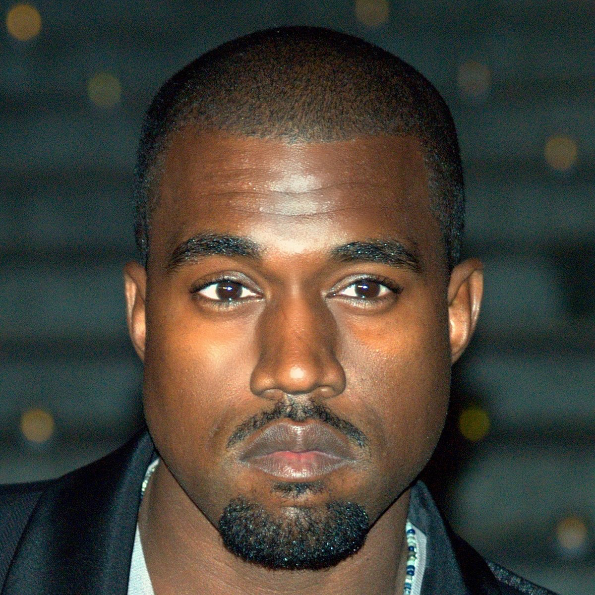
cosine similarity: 0.1
softmax: 2.85%

[0.3,0.1,-0.2,0,0.3,-0.5,0.1,0.2,0.7,0,0.3,-0.4,-0.1,0,0.1,0.5,0.5,-0.4,0.1,-0.1,0,0.4,0,-0.4,-0.4,0.4,-0.1,0.3,0.1,0.8,-0.2,0.4,0,0.2,0.2,0.6,0.3,-0.2,0,1.8,0.3,-0.1,-0.4,-0.1,0.3,3.5,0.4,0.3,0.1,0.1,-0.1,0.2,-0.1,-0.4,-0.6,-0.2,-0.1,0.1,0.1,0.1,0.2,-0.1,0.6,0.7,0.2,-0.2,-0.1,0.6,-0.1,0.1,0,0,0,-0.1,0,0,-0.1,0.4,0.2,0.1,0.2,-0.2,0.5,-0.3,0.2,0.3,0.5,0.1,-0.2,-0.4,-0.2,-0.7,-8.6,-0.4,0.3,0,-0.1,0,0.4,-0.4,0.2,0.3,-0.1,0.3,-0.1,0,-0.6,0.3,-0.5,0.3,-0.2,-0.5,0.2,-0.2,0,-0.2,-0.1,-0.2,0.7,0.5,0,0.7,0.3,-0.5,-0.1,0.4,0.1,0.2,0.1,0.2,0.8,0.3,-0.1,1,0.4,0.2,0,-0.4,-0.4,0.4,0,-0.2,-0.4,0,0.3,-0.4,0.1,0.3,-0.3,0,-0.2,-0.3,1.6,-0.2,-0.2,0.1,-0.2,0.1,-0.1,0.5,0.1,-0.4,-0.5,-0.1,0.3,-0.1,0.7,0,-0.1,-0.4,-0.1,-0.2,-0.2,-0.6,0.1,-0.2,0.2,0,0,0.2,0.2,0.2,0.4,0.1,-0.3,-0.2,-0.2,-0.5,-0.2,0.3,-0.4,0.2,0.3,-0.1,0.7,0,-0.5,-0.2,-0.7,0.3,0.1,0,-0.1,-0.1,0,-0.3,0.4,-0.4,0.4,0.8,0.2,0.4,0.2,-0.2,0,0.2,0.1,0.5,0.4,0.2,-0.3,0.6,-0.2,0.2,0.1,-0.5,0.3,-0.6,-0.3,-0.3,-0.5,0.4,-0.1,-0.1,0.2,0.7,0.2,0.1,0.3,0.2,0,0.5,0,0.5,-0.2,0.3,-0.2,-0.2,0.1,0.6,-0.1,-0.1,0.3,0,0.2,0.4,0,0,-2.2,0.3,0,0.1,0.2,-0.6,0,0,0,0.6,0.1,0,0.2,0.7,0.3,0.3,0.1,0.1,-0.1,0.1,0,-0.7,-0.1,0.1,0.1,0,-0.1,0.1,0.4,-0.2,0,0,0,-0.2,0.1,-0.3,0.2,0,0.2,0.4,0.1,-0.1,0,0.1,-0.4,0.3,-0.2,0.1,0.5,-0.2,0.2,0,0.1,0.5,1,-0.1,0.6,0.1,0.2,-0.1,-0.2,-0.9,0.6,-0.8,-0.2,-0.2,-0.1,0,-0.3,-0.3,0.6,0.1,0,-0.3,0.2,0,0.2,0,0.3,0.7,-0.3,0.2,-0.2,-0.4,0,0.5,0,-0.1,-0.1,-0.1,0.5,0.2,-0.1,0.1,0.2,-0.1,-0.2,-0.5,-0.4,-0.6,0.3,-0.1,0.4,0,-0.3,0.3,0.2,-0.3,-0.2,-0.5,0.2,-0.1,-0.2,0.4,0.4,-0.3,-0.3,0.3,0,0,-0.6,0.1,0.2,-0.3,0.1,0.4,-0.1,-0.1,-0.2,-0.3,-0.3,-0.7,-1,-0.2,-0.5,-0.3,-0.2,0,-0.1,0,0,-0.3,0.2,-0.2,-0.2,-0.1,0.1,-0.1,-0.2,-0.1,0.8,0,0.7,0.4,0.5,0,-0.3,-0.1,0.2,-0.1,0.1,-0.2,-0.2,-0.3,0.1,0.2,0.2,0.1,0.3,-0.1,-1,-0.1,-0.3,0.2,0.7,-0.1,0.2,0.2,0.2,-0.2,0,0.3,0,0,0.3,-0.3,0.3,-0.2,0,0.4,0.1,-0.2,0.4,0.2,-0.1,-0.1,0,-0.3,0.1,-0.2,0.4,-0.3,-0.2,0.3,-0.3,-0.1,0.5,0.5,0,-0.1,-0.3,-0.3,-0.1,0.4,-0.2,-0.4,0,-0.1,-0.3,0.1,-0.2,-0.1,0.3,0,-0.1,0.1,-0.1,-0.3,-0.4,0.4,-0.4,-0.1,-0.1,0.1,0.5,0.1,-0.1,-0.2,-0.2,0.5,0.3,0.1,0,0,0.1,-0.2,0.7,0.1,-0.2,0.1,-0.2,0.9,0.1,-0.2]

cosine similarity: 0.08
softmax: 2.3%

[0,-0.2,0,-0.2,-0.1,-0.1,-0.5,0.3,-0.3,-0.1,0.1,0.1,-0.4,0,-0.1,0.3,-1.2,-0.3,0,0.3,0.2,0.2,-0.5,0,0.1,0.3,0.3,0,-0.2,-0.4,-0.2,-0.8,-0.1,0.1,0.9,0.2,-1,0.3,-0.1,0.2,0,0.1,0.1,-0.3,-0.4,-0.3,-0.1,-0.1,-0.5,0.7,0.1,0.3,-0.2,-0.1,-0.2,0,0.2,0.2,-0.2,-0.2,0.2,-1,0.2,0.1,-0.3,0,0,0,0.2,0,0.3,-0.5,-0.2,-0.2,-0.4,0.1,-0.4,-0.4,0,0.2,-0.1,0.2,-0.2,-0.1,0.3,0.1,1,0.2,-0.1,-0.1,0.1,0,-5,0.6,0.1,0.5,0,0,-0.5,-1.9,0.2,0,0.5,-0.1,0.6,0.1,-1.6,0.3,0.3,-0.3,-0.7,-0.6,0,0,-0.2,0.5,0.2,-0.2,-0.2,0.4,0.1,0.6,0.6,-0.1,-0.3,0.1,-0.4,-0.3,-0.4,0.4,-0.4,0.1,-0.3,0.8,-0.2,0.2,0.1,-0.5,0.4,0,-0.1,0.3,-0.3,-0.3,-0.1,0.1,-0.3,0.3,0.4,-0.2,0.6,0.3,1.3,-0.3,0.3,-0.3,-0.1,-0.4,-0.4,-0.3,-0.3,0.1,-0.2,-0.8,-0.4,-0.7,1.6,0,-0.4,-0.2,0.6,0.4,0.7,0.2,0.3,0.5,-1.4,-0.4,0.1,0.1,-0.6,0,-0.8,-0.8,-0.2,-0.5,0.4,-0.5,-0.1,-0.2,-0.3,-0.6,0.1,0.1,0.8,0.1,0.3,0.5,-0.5,0,0,0,0.3,-0.2,0.3,-0.4,0.2,0,-0.2,0.3,-0.1,-0.2,0.1,0.2,-0.2,0.3,0.4,-0.2,-0.3,-0.3,-0.2,0.6,-0.1,-0.4,-0.4,-0.4,0,-0.2,0.2,0.6,0.4,-0.3,-0.1,0.5,-0.3,0.2,0.1,0,0.1,-0.2,0.1,0.4,0.5,-0.6,0.2,0.5,0.5,0.3,0.1,-0.6,-0.4,0.4,0.2,0.1,0.7,0,-0.1,-0.1,0,-0.2,-0.5,0.1,-0.5,0.4,0.3,0.1,0.4,0.1,-0.1,-0.4,0.2,0.3,0.4,-0.3,0,0.1,0,0.3,-0.3,0.2,0,0.4,-0.5,0.3,0,0.2,-1.4,0.1,-0.6,0.1,0,0.9,0.1,-0.1,0.1,-0.1,1,0.2,0.6,0.5,0,0.5,-0.2,0.1,0.7,-0.5,0.6,0.5,0,0.7,-0.4,0.3,0.8,-0.1,0.3,0.2,0.2,-0.8,0.4,0.3,-0.4,-0.3,-0.4,-0.1,-0.2,0.1,-0.1,0.3,-0.3,-0.6,0,0,0,0.1,-0.3,0.1,-0.1,0.3,0.4,0.1,-0.2,0.1,-0.5,0.1,0,-0.1,0.7,-0.1,0,0.1,-0.8,0.2,0.4,0.1,-0.1,0.6,-0.2,-0.2,0.1,-0.2,-0.4,-0.1,-0.5,0,-1,0.2,0.1,-0.6,-0.3,-0.1,0.2,0.2,0.3,0.1,-0.3,-0.3,-0.8,-0.2,0.4,0.3,0.1,-0.1,0,0.1,0.2,-0.3,0,-0.4,0.1,0,0,0.2,0.2,-0.3,0.4,0.3,-0.2,0.4,0.1,0,-0.1,-0.5,0.2,0,0.6,-0.4,-0.7,0.2,0.1,0,-1,-0.4,0.4,-0.3,-0.2,0.2,0.3,0.1,0,-0.2,0.2,-0.2,0,-0.3,0.4,0.2,-0.6,-0.2,-2,0,0.2,0,0.6,0.1,-0.4,-0.1,0.1,0.5,0.5,0.1,0,0.4,-0.2,0,0,0,-0.4,-0.1,0.1,0.3,-1,0,0,0.1,0.2,-0.1,0.5,0,-0.1,0,-0.4,0.3,-0.1,-0.4,0.1,0.1,0,0,0.3,-0.1,-0.3,-0.2,0.2,0.4,0.2,0.3,0.2,0,0.2,0.5,-0.3,-0.7,0,0,0.3,0,0,0.4,-0.5,-0.1,-0.1,-0.3,-0.1,-0.2,-0.3,-0.1,-0.3,-0.2,0.2,-0.4,0.2,0,0.1,0.1,0.5,-0.1,0,0,-0.2,-0.4,-0.3,-0.2]

GO

[0.07,0.02,0.01,0.04,0,-0.12,-0.03,0.03,-0.06,-0.06,-0.03,-0.04,0.02,-0.02,0,0.08,-0.02,-0.05,-0.02,-0.04,0,-0.01,0.03,-0.01,0.02,0.02,0.03,-0.02,0.03,-0.02,0.07,0.06,-0.03,-0.06,-0.03,-0.02,-0.01,-0.04,0.03,0,-0.09,-0.02,0,0,0,-0.02,-0.02,0.01,-0.07,0.01,0.02,0,-0.02,0.01,0.02,0.01,-0.02,0.07,-0.05,-0.01,-0.02,0,0.02,0.04,-0.04,-0.05,-0.04,0.03,0,0.01,-0.02,0,0.05,0,-0.06,0.03,0.01,0.03,-0.06,0,0.01,0.04,-0.01,-0.04,0.03,0,-0.02,-0.05,-0.02,0.04,-0.02,0,-0.07,0.06,0,-0.04,0.03,0.04,0,-0.1,0.04,0.04,0.07,0,0.02,0.05,0,-0.05,-0.01,0,-0.04,0.11,-0.01,0,-0.02,-0.01,-0.03,-0.04,-0.04,0.04,0.04,-0.2,-0.01,-0.08,0.06,-0.04,0.02,0.02,-0.03,0.01,0.02,-0.01,-0.06,0.21,-0.04,-0.06,-0.03,-0.05,0.03,-0.06,-0.05,0.03,-0.04,-0.05,-0.07,-0.04,-0.04,-0.01,-0.05,0.01,0.01,0.01,0.01,0.05,0.02,0.04,0.04,-0.04,-0.04,0.01,-0.01,0.05,-0.04,0.03,0.04,0.01,0,-0.02,-0.05,0.04,0,0.01,-0.03,-0.03,0.01,0.05,0.02,-0.01,0.02,-0.02,-0.02,0.02,0.01,-0.04,0,-0.03,0.06,-0.04,-0.05,0.05,-0.03,0.02,0.04,-0.03,-0.04,0,0.07,0.01,0.03,-0.04,-0.01,0.04,0,-0.03,-0.03,-0.06,0.01,0.01,-0.01,-0.07,0.03,-0.02,0.01,0.07,-0.01,0.04,-0.01,0.04,0.04,-0.01,-0.03,0.01,0.03,0,0.02,-0.01,0.03,-0.04,0.01,0,0.06,0.04,0.02,0.07,-0.01,-0.04,0,-0.04,-0.07,-0.05,-0.02,0.07,0.02,0.05,-0.02,-0.02,0.03,-0.05,0.01,0.05,-0.09,-0.04,0,0.09,0,0.01,0.05,0.01,-0.01,0.01,-0.07,0.03,0.07,-0.04,0.03,0.02,-0.01,-0.08,-0.08,0.06,-0.02,0,0.05,0.07,-0.01,-0.01,0.01,-0.03,0,0.02,-0.03,0.08,0.07,-0.03,0.03,-0.01,0,-0.05,0.04,-0.02,0,0.03,-0.07,0.04,-0.05,-0.01,-0.03,0,0.08,-0.02,-0.01,0.01,0.02,0.01,0.04,-0.09,0.03,0.05,0.01,-0.05,-0.06,0,0.21,0.04,0.09,-0.04,0.03,0.08,-0.03,-0.03,0.05,0.05,0.01,0.04,-0.04,0.04,0.04,0,0.03,0.05,0.04,-0.02,0.03,-0.03,0.02,-0.04,0.01,0.06,0.05,0.02,0.05,0.01,-0.01,-0.04,0.05,-0.02,0.06,0,-0.06,-0.08,-0.02,0,-0.01,0.07,0,0.07,0.05,-0.05,0.02,-0.04,0.1,0.01,-0.04,0.1,0.01,0,0.03,0.01,0,-0.05,-0.07,-0.05,-0.02,0.02,0.08,-0.01,0,-0.01,-0.1,0.01,-0.02,0,0.02,-0.04,-0.02,-0.03,-0.04,-0.03,0.04,-0.06,-0.07,0.03,0,0.02,0.09,-0.04,-0.02,0.05,-0.01,0.09,0.03,0.02,0.02,0,-0.02,0,-0.04,-0.06,0.05,0,0.09,-0.03,-0.04,0.01,-0.03,0.04,-0.03,-0.07,0.03,0.04,0.11,-0.01,0.08,-0.11,0.06,0.02,-0.06,0.03,0.04,-0.01,0.02,0.03,0.01,-0.06,0,-0.07,-0.08,0.05,-0.01,0.02,-0.01,-0.04,0.01,-0.06,-0.01,0.02,-0.06,0.01,-0.03,0.04,-0.03,0.03,-0.01,-0.05,0.03,-0.06,0.02,-0.03,0.02,0,-0.04,0.04,-0.03,0.02,0.05,-0.01,-0.04,0.02,0.02,0.01,0.07,-0.01,0.03,-0.03,0.04,0.04,-0.06,-0.04,0.01,0.02,-0.01,0.12,0.04,0.03,-0.02,-0.03,-0.05,0.01,0.01,-0.02,-0.05,0,-0.02,-0.02,0.06,-0.11,0.13,0.03,-0.06,-0.03,0.02,-0.01,-0.01,0.06,0.1,0.08,-0.01,-0.02,0.03,0.1,-0.04,0.01]

show embeddings

This ability to match text and images is incredibly powerful and can be used to perform a vast array of vision tasks. CLIP can be used to classify an image by calculating the similarity scores between an image and the phrase: "a photo of {class name}", then choosing the class with the highest similarity score.

With slightly more work, the similarity score that CLIP calculates can be used for many other tasks, such as image captioning or object detection.

How CLIP Works

There are 3 main components of CLIP: the similarity metric, the text encoder, and the image encoder.

Let's start with the similarity metric. Given two vectors, we can measure their similarity by the cosine of the angle between them. See the 2-dimensional visualization below.

Let's consider 2 vectors $x$ and $y$, which an angle $\theta$ between them. If $x$ and $y$ are very similar, then $\theta$ will be small and $\cos(\theta)\approx 1$. If $x$ and $y$ are roughly orthogonal, then $\theta$ will be approximately $90$ degrees and $\cos(\theta)\approx 0$. If $x$ and $y$ are in opposite directions, then $\theta$ will be very large ($\approx 180$ degrees) and $\cos(\theta)\approx -1$. This is the similarity metric that CLIP uses.

The difficulty comes with embedding the image and text. In order to calculate the similarity score between text and an image, it must have an equal-dimension vector representation of each. And, more importantly, in order for the cosine similarity score to produce meaningful values, CLIP must ensure that the vector representations are aligned such that similar concepts have similar vectors. For example, the vector representing an image of a dog should be similar to the vector representing the sentence, "the dog barked."

CLIP addresses the challenge of embedding the image and text to a same dimension vector by using a transformer to embed the text into a 512-dimensional vector, and a vision transformer to embed the image into a 512-dimensional vector. We will not explain transformers or vision transformers, but you can read this article for an explanation of transformers and the seminal vision transformer paper for their explanation.

Training

Of course, an untrained transformer's embedding of images and text will be meaningless. In order to teach the model to align the text and image embeddings, CLIP is trained on lots of data -- nearly 400 million pairs of images and text. These image-text pairs are found "in the wild", meaning that they could be an image and its caption on instagram, or an image and its description on Wikipedia.

CLIP does not employ the typical strategy of using a network to exactly predict the text from the image. For these "in the wild" text-image pairs, the text is far too varied to be predicted exactly. So, instead, CLIP's training objective maximizes the cosine similarity between true text-image pairs, and minimizes the similarity between false text-image pairs.

This idea is shown below, where $N$ is the number of examples in a batch, and $T_i$ is the text encoding of the $i$'th caption in the batch, and $I_i$ is the image encoding of the $i$'th image in the batch.

Concretely, for each training update, 32,768 image-text pairs are randomly sampled from the dataset. Then, the model encodes both the text and the image, and calculates the cosine similarity for each possible text-image pair.

If CLIP was perfect, then the cosine similarity for the true text-image pair will be higher than any other text-image pair. So, in the cosine similarity matrix, the diagonal values should be as high as possible, and the non-diagonal values should be as low as possible. CLIP embeds this in the training signal by using cross-entropy loss where the correct label is the diagonal. In order to be more robust to the noisy labels, the authors of CLIP opted to use a variant of cross-entropy loss called symmetric cross-entropy loss, which you can read about here.

You now understand how we can connect text and images using CLIP! Feel free to play around with the CLIP tool at the top of this section. You can see the cosine similarity between any text prompt and the four given images, each image's embedding, and your prompt's embedding. Now, we will go over a model which can generate images from random noise.

GANs

A Generative Adversarial Network (GAN) is a model that creates realistic-looking images (it can create other types of data, but we are interested in image-producing GANs). For example, visit thispersondoesnotexist.com to see examples of a GAN trained to produce realistic-looking faces.

How does it work? It uses a very clever idea: iteratively train two neural networks: one that can distinguish between real images and fake images (the Discriminator), and one that generates fake images to fool the Discriminator (the Generator).

GAN

Randomly sample a vector to feed into the Generator and see the generated image.

Sample from latent space

Training

The Discriminator and the Generator are trained iteratively. In each training iteration, the Discriminator is trained for $k$ steps, then the Generator is trained on a batch of data. In this way, both the Discriminator and the Generator have to continue to improve in order to keep pace with the other.

Generator Loss Function

In order to create images, the generator takes as input a vector of random noise $Z$. Then, the goal of the generator $G$ is to create an image $G(z)$ from this noise that fools the discriminator $D$. The generator fools the discriminator if the discriminator assigns high probability to the generated image being real.

So, the generator wants to minimize the expression $\mathbb{E}_{x\sim p_z(x)}[\log(1-D(G(z)))]$. If the discriminator is fooled, then $D(G(z))$ will be close to 1, so $\mathbb{E}_{x\sim p_z(x)}[\log(1-D(G(z)))]$ will be very negative. If the discriminator is not fooled, then $D(G(z))$ will be close to 0, so $\mathbb{E}_{x\sim p_z(x)}[\log(1-D(G(z)))]$ will be close to 0.

Discriminator Loss Function

A perfect discriminator should always assign 100% probability that a real image $x$ is real. So, given some data-generating process $p_{data}(x)$, we want a discriminator that maximizes the expression $\mathbb{E}_{x\sim p_{data}(x)}[\log D(x)]$.

A perfect discriminator would also assign 0% probability that an image generated by the generator $D(G(z))$ is real. So, the discriminator should maximize the expression that the generator was minimizing: $\mathbb{E}_{x\sim p_z(x)}[\log(1-D(G(z)))]$.

So, a discriminator that wants to correctly classify both real and fake images should maximize the expression $\mathbb{E}_{x\sim p_{data}(x)}[\log D(x)] + \mathbb{E}_{x\sim p_z(x)}[\log(1-D(G(z)))]$.

Complete Training

Now that we have the function the Generator wants to maximize: $$\mathbb{E}_{x\sim p_z(x)}[\log(1-D(G(z)))]$$ and the function the Discriminator wants to minimize: $$\mathbb{E}_{x\sim p_{data}(x)}[\log D(x)] + \mathbb{E}_{x\sim p_z(x)}[\log(1-D(G(z)))]$$ we can formulate the loss function for each and run gradient descent. This is all there is to training a GAN (well, in reality, there are many tricks that are necessary to avoid mode collapse and make sure that the training goes smoothly)!

CLIP + GAN

Now that we understand CLIP -- which can connect text and images -- and GANs -- which can create realistic images -- how can we connect them to create images from text?

Using the similarity score produced by CLIP, we can evaluate how close a GANs output is to a given text prompt. So, we can use CLIP to guide a GAN towards producing an image that is most similar to the text input!

CLIP + VQGAN

"A painting of a red telephone box spinning through a time vortex"

Loss function

If we use the Generator from a large pre-trained GAN (such as BigGAN or VQGan), then when we sample from the latent space $z\sim Z$ and produce an image $G(z)$, it will seem fairly natural. We can encode this image $G(z)$ using CLIP to create an image encoding $i$, encode the text prompt $T$ to create a text encoding $t$, and calculate their similarity $s(i, t)$ using cosine similarity. We want to change $G$ and $z$ to maximize $s(i, t)$.

So, we can use $-s(i, t)$ as the loss function, and backpropagate the loss through the GAN and latent space.

This procedure is unique because it resembles a typical training procedure, but it is being used for inference. Each time we want to make art, we need to run backpropagation through the GAN and latent space. Due to this optimization at inference, generating images is slow. Here are a few Google Colabs where you can generate images from GANs/other generative models:

• VQGAN + CLIP
• BigGAN + CLIP
• Deep Daze

CLIPDraw

We don't necessarily have to use a GAN to create images with CLIP. We could randomly generate pixels, calculate the similarity score with CLIP, then backpropagate through everything and update the pixels to produce an image that has a high similarity score. However, this often leads to images that are very noisy and uninteresting. By restricting ourselves to the latent space of the GANs, we are introducing a "natural image prior" that constrains the image, roughly, to images that look like real objects.

We can introduce a "natural image prior" without a GAN. In CLIPDraw, they constrain the space of images to images produced by strokes of color. Technically, "CLIPDraw uses a differentiable renderer as a representation for generating drawings; namely a set of RGBA Bezier curves are optimized rather than a matrix of pixels."

CLIPDraw initializes a scene with randomly initialized Bezier curves. Then, at each optimization step, uses the cosine similarity as the loss function (similarly to the CLIP + GAN case), and runs backpropagation through the vector graphics space.

CLIPDraw

Watercolor painting of an underwater submarine.

Continuing From Here

We've explored CLIP, GANs, and their combination: what each does, how it is trained, and why it is interesting.

To learn about the origins of connecting CLIP with GANs to create art, see this blog post.

I hope you learned something, found it interesting, and will make art using CLIP. If you do, please email me! I'm excited to see what you come up with.